A R Basics

A.1 Get R and RStudio

First download and install R from https://cran.r-project.org.

Then, download and install RStudio (Desktop) from https://posit.co/products/open-source/rstudio/.

(You should have permission for both of these. If not, you may need to contact EOM IT.)

A.2 Read in data files

We can read data from many formats and many places, including from a local file or from the web. Many R packages contain their own data.

The code below requires the following packages to be loaded and attached:

library(dplyr)
library(ggplot2)
library(here)
library(lubridate)
library(magrittr)
library(readr)

A.2.1 `.csv`

Data from the web (from the résumé audit experiment from Bertrand and Mullainathan (2004)):

df_resume <- read_csv("https://raw.githubusercontent.com/kosukeimai/qss/master/CAUSALITY/resume.csv")

Then we can examine the dimensions of the new object named df_resume:

dim(df_resume)

## [1] 4870    4

So, df_resume has 4870 rows and 4 columns. We can see the first few rows with

head(df_resume)

## # A tibble: 6 × 4
##   firstname sex    race   call
##   <chr>     <chr>  <chr> <dbl>
## 1 Allison   female white     0
## 2 Kristen   female white     0
## 3 Lakisha   female black     0
## 4 Latonya   female black     0
## 5 Carrie    female white     0
## 6 Jay       male   white     0

For data from a local file, if data mydata.csv are in subdirectory /data/,

my_data_path <- here("data", "mydata.csv")

df <- read_csv(my_data_path)

See here for more detail on how to use here() to create paths.

A.2.2 `.xlsx`

Use package readxl and function read_excel(). To read the second sheet from a multi-sheet spreadsheet, add an argument like read_excel(..., sheet = 2).

A.2.3 Box

To read a file directly from box, we use the boxr package. To do so,

Have a member of the data science team (currently, Nathan) add you as Box RStudio App collaborator
Go to dcgov.box.com. At the bottom left, click “Dev Console”
Click on The Lab @ DC
Click the Configuration tab

Here you should see a client_id and client_secret that you can copy.

Then, run at the R Console

library(boxr)

box_auth(client_id = "<INSERT ID STRING HERE>",
         client_secret = "<INSERT SECRET STRING HERE>")

replacing the strings with the information from the Configuration tab.

If R prompts you to update the Renviron file to store this information for next time, you may do so.

Then, your .R file that reads the data should include

library(boxr)

box_auth() 
# (arguments can be empty, if credentials stored in Renviron)

df <- box_read("791112121820")
# (where 791112121820 is the Box ID for a .csv to read)

For more information, see the boxr vignette.

A.3 Pipes

Pipe operators make it easier for humans to follow a code chunk, and they allow us to string together a sequence of operations into a “pipeline”. The native R pipe is |>; the pipe from package magrittr is also very common (%>%).

The pipe simply takes the argument on its left and passes it as the first argument of the function to its right. So, if I have function f() to which I will pass arguments x and y (in that order), I can write

f(x, y)

Using a pipe, I can equivalently write either

x |> f(y)

x %>% f(y)

A.4 Rename variables

Variable names should adhere to good practices.

The rename() function in dplyr can rename several variables at once:

df <- df |> rename(new_var_name_1 = `Bad, old, long, spacey name`,
                    new_var_name_2 = "inconsistentsquishedvarname",
                    new_var_name_3 = starts_with("Unique string old name starts with"))

To automatically clean up all the names in a dataframe, the {janitor} package can help:

df <- df |> clean_names()

A.5 Create a New Variable

Suppose I want to create a new variable and attach it to the data frame (i.e., to update the data frame to include the new variable). Mechanically, in the tidyverse I overwrite the old data frame with the new one. Sometimes we want to use a new name for the augmented data frame, but not when we create each new variable.

A.5.1 Create a “wave ID”

A “wave ID” is a variable that is constant for every row in the data set. Suppose that the resume data were all from “wave 3” of a larger study. To identify them as such,

df_resume <- df_resume |> mutate(wave = 3)

A.5.2 Create a primary key

A “primary key” is a variable that uniquely identifies each row in the data set. To create a primary key or “ID variable”,

df_resume <- df_resume |> mutate(id_var = row_number())

A.5.3 Transform an existing variable

Below, we use the mutate() function with the character variable sex, which has levels female and male, to create a logical TRUE/FALSE variable indicating whether the résumé had a putatively female name at the top:

df_resume <- df_resume |> mutate(isFemale = sex == "female")

Now, df_resume has 7 columns:

head(df_resume)

## # A tibble: 6 × 7
##   firstname sex    race   call  wave id_var isFemale
##   <chr>     <chr>  <chr> <dbl> <dbl>  <int> <lgl>   
## 1 Allison   female white     0     3      1 TRUE    
## 2 Kristen   female white     0     3      2 TRUE    
## 3 Lakisha   female black     0     3      3 TRUE    
## 4 Latonya   female black     0     3      4 TRUE    
## 5 Carrie    female white     0     3      5 TRUE    
## 6 Jay       male   white     0     3      6 FALSE

Note that mutate() needs a dataframe as its first argument. Above, we pass df_resume to mutate() using the pipe.

A.5.4 Create a sum from a subset of variables

Below, we select a subset of columns from df_resume, take the sum across them, and add the sum as a new variable. Here, we locate the new variable right after those columns that it summed.

df_resume |> 
  mutate(new_sum = rowSums(select(df_resume, call:id_var))) |> 
  relocate(new_sum, .after = id_var)

## # A tibble: 4,870 × 8
##    firstname sex    race   call  wave id_var new_sum isFemale
##    <chr>     <chr>  <chr> <dbl> <dbl>  <int>   <dbl> <lgl>   
##  1 Allison   female white     0     3      1       4 TRUE    
##  2 Kristen   female white     0     3      2       5 TRUE    
##  3 Lakisha   female black     0     3      3       6 TRUE    
##  4 Latonya   female black     0     3      4       7 TRUE    
##  5 Carrie    female white     0     3      5       8 TRUE    
##  6 Jay       male   white     0     3      6       9 FALSE   
##  7 Jill      female white     0     3      7      10 TRUE    
##  8 Kenya     female black     0     3      8      11 TRUE    
##  9 Latonya   female black     0     3      9      12 TRUE    
## 10 Tyrone    male   black     0     3     10      13 FALSE   
## # ℹ 4,860 more rows

A.6 Recode a variable’s values

Instead of creating a new variable as above, we can use mutate() and case_when() to recode a variable. Suppose we wanted to code race:

df_resume |> mutate(
  race = case_when(
    race == "white" ~ "race_wh",       # recode "white" to "race_wh"
    race == "black" ~ "race_bl",       # recode "black" to "race_bl"
    race == "missing" ~ NA_character_, # recode "missing" to (character) NA
    TRUE ~ race                        # recode any other value to original value of race
  )
)

## # A tibble: 4,870 × 7
##    firstname sex    race     call  wave id_var isFemale
##    <chr>     <chr>  <chr>   <dbl> <dbl>  <int> <lgl>   
##  1 Allison   female race_wh     0     3      1 TRUE    
##  2 Kristen   female race_wh     0     3      2 TRUE    
##  3 Lakisha   female race_bl     0     3      3 TRUE    
##  4 Latonya   female race_bl     0     3      4 TRUE    
##  5 Carrie    female race_wh     0     3      5 TRUE    
##  6 Jay       male   race_wh     0     3      6 FALSE   
##  7 Jill      female race_wh     0     3      7 TRUE    
##  8 Kenya     female race_bl     0     3      8 TRUE    
##  9 Latonya   female race_bl     0     3      9 TRUE    
## 10 Tyrone    male   race_bl     0     3     10 FALSE   
## # ℹ 4,860 more rows

There is also recode(), but its lifecycle status is “questioning”:

df_resume |> mutate(
  race = recode(race,
    "white" = 0,
    "black" = 1
    )
)

## # A tibble: 4,870 × 7
##    firstname sex     race  call  wave id_var isFemale
##    <chr>     <chr>  <dbl> <dbl> <dbl>  <int> <lgl>   
##  1 Allison   female     0     0     3      1 TRUE    
##  2 Kristen   female     0     0     3      2 TRUE    
##  3 Lakisha   female     1     0     3      3 TRUE    
##  4 Latonya   female     1     0     3      4 TRUE    
##  5 Carrie    female     0     0     3      5 TRUE    
##  6 Jay       male       0     0     3      6 FALSE   
##  7 Jill      female     0     0     3      7 TRUE    
##  8 Kenya     female     1     0     3      8 TRUE    
##  9 Latonya   female     1     0     3      9 TRUE    
## 10 Tyrone    male       1     0     3     10 FALSE   
## # ℹ 4,860 more rows

A.7 Treat dates as dates

When we have dates stored as character strings, we transform them to dates. First, simulate some date data:

# Simulate date data:
set.seed(117894985)

df_resume <- df_resume |> 
  mutate( 
    dob = paste0(sample(1:12, n(), replace = TRUE), 
                 "/", 
                 sample(1:28, n(), replace = TRUE),
                 "/",
                 sample(1950:2000, n(), replace = TRUE))
)

head(df_resume, 3)

## # A tibble: 3 × 8
##   firstname sex    race   call  wave id_var isFemale dob      
##   <chr>     <chr>  <chr> <dbl> <dbl>  <int> <lgl>    <chr>    
## 1 Allison   female white     0     3      1 TRUE     1/28/1994
## 2 Kristen   female white     0     3      2 TRUE     2/15/1983
## 3 Lakisha   female black     0     3      3 TRUE     1/10/1977

The tidyverse includes the lubridate package. If you know the format of the character strings, there are many shortcut parsers like mdy(). Below, we recode character dates to be of date type:

df_resume |> mutate(
  dob_date = mdy(dob)
)

## # A tibble: 4,870 × 9
##    firstname sex    race   call  wave id_var isFemale dob        dob_date  
##    <chr>     <chr>  <chr> <dbl> <dbl>  <int> <lgl>    <chr>      <date>    
##  1 Allison   female white     0     3      1 TRUE     1/28/1994  1994-01-28
##  2 Kristen   female white     0     3      2 TRUE     2/15/1983  1983-02-15
##  3 Lakisha   female black     0     3      3 TRUE     1/10/1977  1977-01-10
##  4 Latonya   female black     0     3      4 TRUE     2/28/1985  1985-02-28
##  5 Carrie    female white     0     3      5 TRUE     5/1/1957   1957-05-01
##  6 Jay       male   white     0     3      6 FALSE    11/2/1964  1964-11-02
##  7 Jill      female white     0     3      7 TRUE     10/25/1954 1954-10-25
##  8 Kenya     female black     0     3      8 TRUE     2/18/1963  1963-02-18
##  9 Latonya   female black     0     3      9 TRUE     12/18/1980 1980-12-18
## 10 Tyrone    male   black     0     3     10 FALSE    7/25/1956  1956-07-25
## # ℹ 4,860 more rows

If we aren’t sure of the format, or there are several, we use parse_date_time() and specify several “orders” of date format. parse() functions do their best to use the information in “orders”. Below, "dmy" alone would recode only the ambiguous dates, assuming they were in day-month-year order. Adding "%m/%d/%Y" instructs parse() to look for month/day/year formats. Finding many that are unambiguously that format, it assumes that format for the new variable.

df_resume |> mutate(
  dob_date = as_date(    
    parse_date_time(dob, 
                    orders = c("dmy", "%m/%d/%Y"))
  )
)

## # A tibble: 4,870 × 9
##    firstname sex    race   call  wave id_var isFemale dob        dob_date  
##    <chr>     <chr>  <chr> <dbl> <dbl>  <int> <lgl>    <chr>      <date>    
##  1 Allison   female white     0     3      1 TRUE     1/28/1994  1994-01-28
##  2 Kristen   female white     0     3      2 TRUE     2/15/1983  1983-02-15
##  3 Lakisha   female black     0     3      3 TRUE     1/10/1977  1977-01-10
##  4 Latonya   female black     0     3      4 TRUE     2/28/1985  1985-02-28
##  5 Carrie    female white     0     3      5 TRUE     5/1/1957   1957-05-01
##  6 Jay       male   white     0     3      6 FALSE    11/2/1964  1964-11-02
##  7 Jill      female white     0     3      7 TRUE     10/25/1954 1954-10-25
##  8 Kenya     female black     0     3      8 TRUE     2/18/1963  1963-02-18
##  9 Latonya   female black     0     3      9 TRUE     12/18/1980 1980-12-18
## 10 Tyrone    male   black     0     3     10 FALSE    7/25/1956  1956-07-25
## # ℹ 4,860 more rows

A.7.1 Make an age variable

To make an age variable from the year component,

df_resume |> mutate(
  age = 2023 - year(dob_date)
)

## # A tibble: 4,870 × 10
##    firstname sex    race   call  wave id_var isFemale dob       dob_date     age
##    <chr>     <chr>  <chr> <dbl> <dbl>  <int> <lgl>    <chr>     <date>     <dbl>
##  1 Allison   female white     0     3      1 TRUE     1/28/1994 1994-01-28    29
##  2 Kristen   female white     0     3      2 TRUE     2/15/1983 1983-02-15    40
##  3 Lakisha   female black     0     3      3 TRUE     1/10/1977 1977-01-10    46
##  4 Latonya   female black     0     3      4 TRUE     2/28/1985 1985-02-28    38
##  5 Carrie    female white     0     3      5 TRUE     5/1/1957  1957-05-01    66
##  6 Jay       male   white     0     3      6 FALSE    11/2/1964 1964-11-02    59
##  7 Jill      female white     0     3      7 TRUE     10/25/19… 1954-10-25    69
##  8 Kenya     female black     0     3      8 TRUE     2/18/1963 1963-02-18    60
##  9 Latonya   female black     0     3      9 TRUE     12/18/19… 1980-12-18    43
## 10 Tyrone    male   black     0     3     10 FALSE    7/25/1956 1956-07-25    67
## # ℹ 4,860 more rows

For more precision, the participants’ ages as of 2 May 2023,

df_resume |> mutate(
  age = as.numeric(
    interval(dob_date, "2023-05-02"), 
    "years")
)

## # A tibble: 4,870 × 10
##    firstname sex    race   call  wave id_var isFemale dob       dob_date     age
##    <chr>     <chr>  <chr> <dbl> <dbl>  <int> <lgl>    <chr>     <date>     <dbl>
##  1 Allison   female white     0     3      1 TRUE     1/28/1994 1994-01-28  29.3
##  2 Kristen   female white     0     3      2 TRUE     2/15/1983 1983-02-15  40.2
##  3 Lakisha   female black     0     3      3 TRUE     1/10/1977 1977-01-10  46.3
##  4 Latonya   female black     0     3      4 TRUE     2/28/1985 1985-02-28  38.2
##  5 Carrie    female white     0     3      5 TRUE     5/1/1957  1957-05-01  66.0
##  6 Jay       male   white     0     3      6 FALSE    11/2/1964 1964-11-02  58.5
##  7 Jill      female white     0     3      7 TRUE     10/25/19… 1954-10-25  68.5
##  8 Kenya     female black     0     3      8 TRUE     2/18/1963 1963-02-18  60.2
##  9 Latonya   female black     0     3      9 TRUE     12/18/19… 1980-12-18  42.4
## 10 Tyrone    male   black     0     3     10 FALSE    7/25/1956 1956-07-25  66.8
## # ℹ 4,860 more rows

(To get participants’ ages today, replace "2023-05-02" above with today().)

A.7.2 Make a month-count variable

We may have dates accurate to the day, but we want a count of which month of participation it is for each participant. Assume that each firstname in the resume data represents a participant, and each dob_date represents an event for that participant that we care about. We want to produce a variable that is 0 for the first month of participation (say, February), and 2 for the month two months later (April), regardless of whether the month between (March) appears in the data, and even if participants start or finish participation at very different times.⁸

Below, we group by firstname, then round all months to the first date of the month, then count those months (within firstname). We show the first three rows for each participant.

df_resume |> 
  # Ensure ranking _within_ firstname:
  group_by(firstname) |> 
  # Round all months to first date of the month, then count:
  mutate(dob_month = floor_date(dob_date, unit = "month"), 
         dob_month_count = (min(dob_month) %--% dob_month) %/% months(1)
         ) |>
  # For presentation, select, arrange, and slice:
  select(firstname, dob, dob_date, dob_month, dob_month_count) |> 
  arrange(firstname, dob_month_count) |> 
  slice(1:3)

## # A tibble: 108 × 5
## # Groups:   firstname [36]
##    firstname dob       dob_date   dob_month  dob_month_count
##    <chr>     <chr>     <date>     <date>               <dbl>
##  1 Aisha     2/4/1950  1950-02-04 1950-02-01               0
##  2 Aisha     5/17/1950 1950-05-17 1950-05-01               3
##  3 Aisha     1/25/1951 1951-01-25 1951-01-01              11
##  4 Allison   3/25/1950 1950-03-25 1950-03-01               0
##  5 Allison   8/9/1950  1950-08-09 1950-08-01               5
##  6 Allison   9/23/1950 1950-09-23 1950-09-01               6
##  7 Anne      2/25/1950 1950-02-25 1950-02-01               0
##  8 Anne      3/4/1950  1950-03-04 1950-03-01               1
##  9 Anne      8/18/1950 1950-08-18 1950-08-01               6
## 10 Brad      1/27/1952 1952-01-27 1952-01-01               0
## # ℹ 98 more rows

If we prefer the first month to be labeled 1 rather than 0, we just replace %/% months(1) with %/% months(1) + 1.

A.8 Create a completely randomised indicator

This uses mutate(), along with the sample() function to create a random vector of Treatment’s and Control’s and attach it to df_resume:

set.seed(317334706)

df_resume <- df_resume |> mutate(
  my_new_treatment_assg = sample(c("Treatment", "Control"), 
                                 size = n(), 
                                 replace = TRUE))

head(df_resume |> select(-isFemale, -dob))

## # A tibble: 6 × 8
##   firstname sex    race   call  wave id_var dob_date   my_new_treatment_assg
##   <chr>     <chr>  <chr> <dbl> <dbl>  <int> <date>     <chr>                
## 1 Allison   female white     0     3      1 1994-01-28 Treatment            
## 2 Kristen   female white     0     3      2 1983-02-15 Control              
## 3 Lakisha   female black     0     3      3 1977-01-10 Treatment            
## 4 Latonya   female black     0     3      4 1985-02-28 Treatment            
## 5 Carrie    female white     0     3      5 1957-05-01 Control              
## 6 Jay       male   white     0     3      6 1964-11-02 Treatment

See also the {randomizr} package for a variety of helpers.

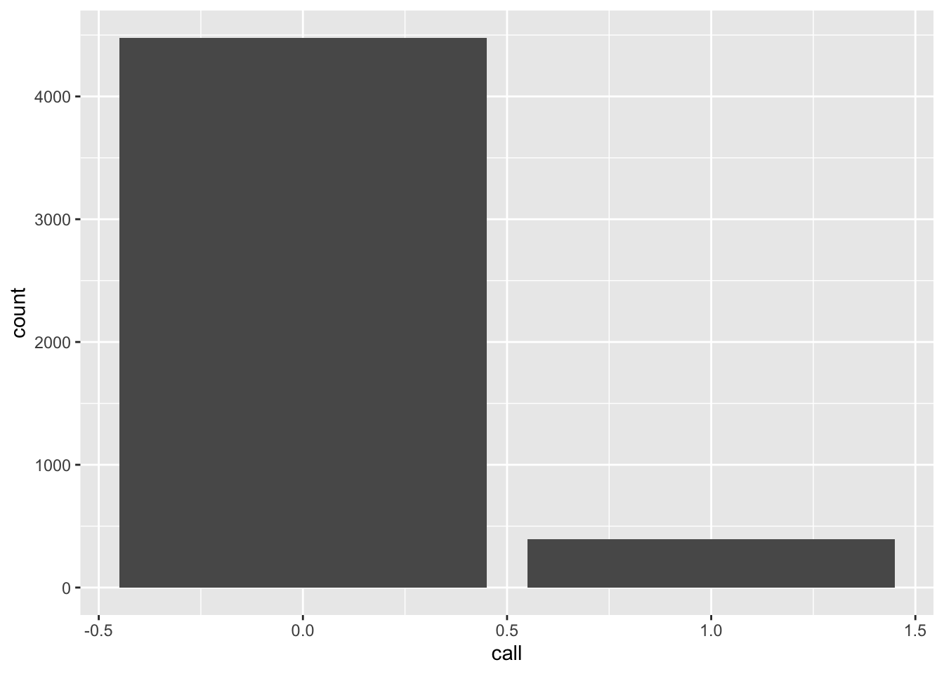
A.9 Plot a variable

Use ggplot() to plot the distribution of calls back that these résumés receive. Calls are fairly rare.

df_resume |> ggplot(aes(x = call)) + geom_bar()

Look at the distribution by the putative race on the resume:

df_resume |> 
  ggplot(aes(x = call, fill = race)) + 
  geom_bar(position = "dodge2")

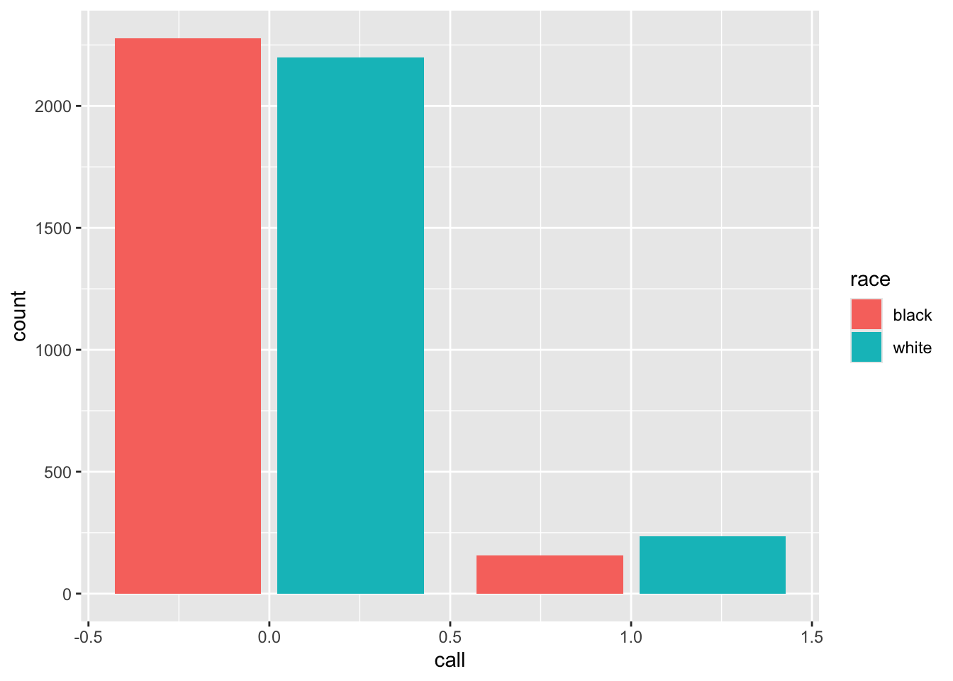
Since there are exactly the same number of résumés with each race, these count distributions are comparable.

A.10 Calculate a data summary

A.10.1 Proportions for a categorical variable

df_resume |> count(firstname) |> mutate(proportion = n / sum(n))

## # A tibble: 36 × 3
##    firstname     n proportion
##    <chr>     <int>      <dbl>
##  1 Aisha       180    0.0370 
##  2 Allison     232    0.0476 
##  3 Anne        242    0.0497 
##  4 Brad         63    0.0129 
##  5 Brendan      65    0.0133 
##  6 Brett        59    0.0121 
##  7 Carrie      168    0.0345 
##  8 Darnell      42    0.00862
##  9 Ebony       208    0.0427 
## 10 Emily       227    0.0466 
## # ℹ 26 more rows

A.10.2 Proportions for binary variables

summ_resume <- df_resume |> 
  group_by(race) |>
  summarise(call_back_rate = mean(call),         # mean of numeric 0/1
            prop_female = mean(sex == "female")) # mean of logical TRUE/FALSE

summ_resume

## # A tibble: 2 × 3
##   race  call_back_rate prop_female
##   <chr>          <dbl>       <dbl>
## 1 black         0.0645       0.775
## 2 white         0.0965       0.764

The call-back rates differ by about 0.032; the proportion female, which will be balanced by the randomization on average, only differs by about 0.011.

A.11 Merge (join) dataframes

For a fuller treatment of merges (“joins”), see here in Wickham and Grolemund (2016).

The four main mutating join commands are left_join(), right_join(), inner_join(), and full_join().

left_join(x, y) keeps all rows of x, but only rows of y that have matches in x
right_join(x, y) keeps all rows of y, but only rows of x that have matches in y
inner_join(x, y) only keeps rows that appear in both x andy
full_join(x, y) keeps all rows of both x and y

For any columns that didn’t appear in the original dataframe for a certain row, the joins will store NA.

By default, joins will match on any columns that have the same name. So, if age and height are both in df1 and df2, then full_join(df1, df2) will consider a row “matched” if the values of both age and height are the same in the datasets.

If column names differ, the by = ... argument can inform the join. E.g., if, instead, df1 has variables Age and Tallness, we could join with

df_joined <- df1 |> full_join(df2, 
                               by = c("Age" = "age",
                                      "Tallness" = "height"))

Columns with the same name, but different types, will not join. E.g., if df1$this_var is numeric, but df2$this_var is character, the joins will throw an error.

A.12 Anonymize sensitive data

Sometimes we want to preserve features of sensitive data, but not the values themselves. For example, we want to match individuals across datasets, but do not want to preserve the individuals’ addresses.

Suppose we have the data below, where each individual has a unique name and phone number, but two share an address:

## # A tibble: 3 × 4
##   Name    Address       Phone Score
##   <chr>   <chr>         <dbl> <dbl>
## 1 Beth    10 Downing St   123    90
## 2 Esme    667 Dark Ave    456    50
## 3 Charles 10 Downing St   789    70

We can anonymize the Address and Phone columns in this data set (called sens) using the digest() function in package {digest}:

library(digest)

cols_to_mask <- c("Address", "Phone")
for(i in cols_to_mask){
  anon <- sapply(unlist(sens[, i]), digest, algo = "sha512")
  
  # Shorten anonymized column (only for presentation here):
  short_anon <- substr(anon, 1, 10)
  
  sens[, i] <- short_anon
}

sens

## # A tibble: 3 × 4
##   Name    Address    Phone      Score
##   <chr>   <chr>      <chr>      <dbl>
## 1 Beth    96aa3d8195 4fb48d053a    90
## 2 Esme    83448c5f34 2145744238    50
## 3 Charles 96aa3d8195 32d3888f19    70

Note that addresses 1 and 3 are the same, despite being hashed.

A.12.1 Salting

Our default one-way procedure is to salt, hash, and key-stretch our sensitive data. Below is an example for a single value we wish to obscure.

library(openssl)

sens <- "1234567"

bcrypt_pbkdf(sens,
             salt = raw(849025))

##  [1] 7c 23 71 da cd 7a 4b f3 3f 70 73 ce 4f 8e 15 a9 77 23 9c b6 d8 8d 85 19 16
## [26] ca 26 c6 88 d4 9a c6

Above, 849025 is a value obtained from sample(1e6, 1) that is used to create the raw salt vector. This value should change for each value we want to hash.

A.13 Deal with factors (ordered/unordered) in models

In typical cases at The Lab, we reorder factor levels to be substantively sorted, but we do not use R “ordered factors”. Reordering makes plotting and regression baselines substantively meaningful; using “unordered” factors ensures that our modeling yields the results we usually desire.

R provides a useful data class called “factors” for categorical variables. See the relevant chapter of Wickham, Çetinkaya-Rundel, and Grolemund (2023) for a full introduction.

We use factors to reorder the groups in a variable. E.g., a simple factor variable sorts its levels in alphabetical order (note the “## Levels:” comment below)

library(forcats)

simple_fct <- factor(rep(c("Low", "Medium", "High"), each = 2))

simple_fct

## [1] Low    Low    Medium Medium High   High  
## Levels: High Low Medium

and thus plots in alphabetical, not substantive, order:

# Make into data frame:
df_factor <- tibble(simple_fct = simple_fct,
                    random_outcome = rnorm(length(simple_fct)))

ggplot(df_factor, aes(simple_fct)) + geom_bar() + labs(x = "A Poorly Ordered Factor")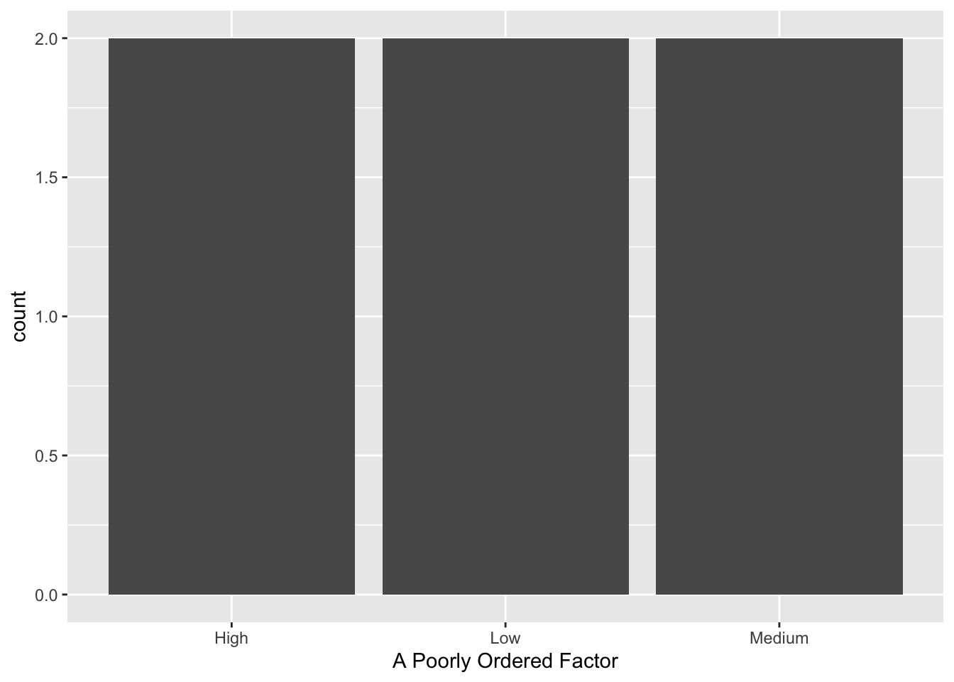

So, we reorder the levels to improve our plotting and give us a better regression baseline category:

df_factor$reordered_fct <-  fct_relevel(simple_fct, 
                                        "Low", "Medium", "High")

df_factor$reordered_fct

## [1] Low    Low    Medium Medium High   High  
## Levels: Low Medium High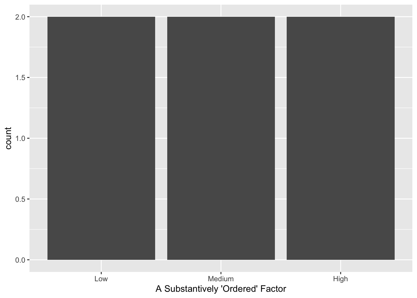

ggplot(df_factor, aes(reordered_fct)) + geom_bar() + labs(x = "A Substantively 'Ordered' Factor")

However, we have not created what R calls an “ordered” factor!

# The factor we reordered is not "ordered":
is.ordered(df_factor$reordered_fct)

## [1] FALSE

To make a factor R-ordered, we would need to set ordered = TRUE:

df_factor$ordered_fct <- factor(df_factor$reordered_fct, ordered = TRUE)

is.ordered(df_factor$ordered_fct)

## [1] TRUE

However, for our typical modeling strategies we use an R-unordered factor (for lm_lin(), lm(), glm(), etc.):

# The "unordered" factor behaves as we usually want.
# We compare levels Medium and High to the baseline:
lm(random_outcome ~ reordered_fct, data = df_factor)

## 
## Call:
## lm(formula = random_outcome ~ reordered_fct, data = df_factor)
## 
## Coefficients:
##         (Intercept)  reordered_fctMedium    reordered_fctHigh  
##             -0.3146               0.1738               1.1078

# The R "ordered" factor does something different:
lm(random_outcome ~ ordered_fct, data = df_factor)

## 
## Call:
## lm(formula = random_outcome ~ ordered_fct, data = df_factor)
## 
## Coefficients:
##   (Intercept)  ordered_fct.L  ordered_fct.Q  
##        0.1126         0.7833         0.3104

Unless we want these exact polynomial contrasts as your results, we avoid R “ordered” factors. Where do these coefficients come from in the “ordered” factor model? See here. For a deeper dive into how R forms the orthonormal basis to create the variables in the “ordered” factor model, see here.

References

Bertrand, Marianne, and Sendhil Mullainathan. 2004. “Are Emily and Greg More Employable Than Lakisha and Jamal? A Field Experiment on Labor Market Discrimination.” American Economic Review 94 (4): 991–1013.

Wickham, Hadley, Mine Çetinkaya-Rundel, and Garrett Grolemund. 2023. R for Data Science (2e). O’Reilly Media, Inc. https://r4ds.hadley.nz.

Wickham, Hadley, and Garrett Grolemund. 2016. R for Data Science: Import, Tidy, Transform, Visualize, and Model Data. O’Reilly Media, Inc. https://r4ds.had.co.nz.

If, instead, we want a variable with 1 for the first date for that participant, 2 for the second date, etc., regardless of how far between the two dates are, we can use dplyr::dense_rank().↩︎